How to assess the level of interest rates ?

The Taylor rate: a frequently used benchmark

The interest rate prescribed by the Taylor (1993)  rule is the most frequently used benchmark for assessing the level of nominal interest rates. What is it? The Taylor rule is a relation that describes the desired short-term interest rate as a function of (i) the deviation of inflation from its target, (ii) a measure of activity (for example, the deviation of output from its potential level or the deviation of unemployment from its "natural" level), and (iii) the so-called "neutral" real interest rate. On this point, see Garnier, Lhuissier et Penalver (2019).

This rule provides a positive description of monetary policy: it describes what has been done. But under certain conditions, it also offers a normative recommendation: it says what should be done. As such, it is often used as the benchmark against which the level of the short-term nominal interest rate should be compared. If the latter is lower (resp. higher) than the level prescribed by the Taylor rule, monetary policy is considered accommodative (resp. restrictive).

The question is therefore not whether interest rates are too low or too high in absolute terms, but rather whether they are above or below the level prescribed by the Taylor rule.

But a benchmark surrounded by great uncertainty

However, this question poses several practical problems.

(1) What is the correct specification of the Taylor rule? There are dozens of alternative formulations, depending on whether the year-on-year or quarterly price change is used, whether the contemporaneous or expected value of the variables is considered, whether or not a measure of the variable neutral rate is included (see the post The natural rate of interest: estimates for the euro area) and depending on the definition of the measure of activity. From one specification to the next, the monetary policy assessment may change considerably.

(2) What are the values of the parameters of the Taylor rule? Assuming that the correct specification of the Taylor rule is known, the values of its parameters have to be estimated and are therefore subject to statistical uncertainty. Again, the monetary policy assessment will change depending on whether the rule responds more or less vigorously to the deviation of inflation from its target.

(3) And even assuming that we know the correct specification and the values of the parameters of the Taylor rule, the question remains as to how to measure the variables of economic activity that the Taylor rule incorporates but that are not directly observable (for example, the output gap or the neutral rate)?

On each of these dimensions, the level of the Taylor rate is subject to considerable uncertainty, as with any macroeconomic assessment. Paraphrasing Christopher Sims, winner of the 2011 Nobel Prize in Economics, the task of economists is to characterise the probability distribution around this level.

Integrating this uncertainty into monetary policy assessment

The correct formulation of a monetary policy assessment must therefore incorporate the uncertainty surrounding the Taylor rate. But how can this be done in practice?

The approach proposed here first consists in obtaining 200 possible specifications of the Taylor rule, broadly covering the scope of the rules considered in the literature since Taylor's paper. These rules are then combined with a simplified representation of the euro area economy, consisting of a demand curve (investment-saving curve or IS curve) and a supply curve (Phillips curve). These two curves are used to identify unobservable variables (natural output, neutral rate).

All these combined relationships form 200 macroeconometric models that are estimated. At the estimation stage it is possible to characterise (1) the probability distributions of the different models; (2) conditional on a model, the probability distributions of the parameters of the different Taylor rules; and (3) conditional on a model and values for its parameters, the probability distributions of the unobservable variables.  

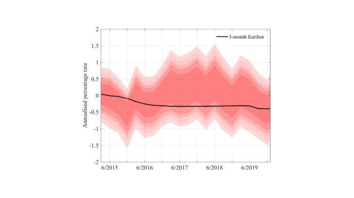
Combining these distributions leads to a characterisation of the uncertainty surrounding the Taylor rate. It is shown in Chart 1, over the period 2014-2019. The black line corresponds to the 3-month Euribor, taken here as the relevant short-term interest rate. The pink areas, from the darkest to the lightest, correspond to the 50%, 70%, 80%, 90% and 95% confidence intervals of the Taylor rates.

In 2019, the euro area short-term interest rate was close to the middle of the probability distribution of Taylor rates.

With very few exceptions (such as at end-2015, just before the ECB's key rate cut in March 2016), the 3-month Euribor is within the 50% confidence interval of Taylor rates (the dark pink area). In particular, in 2019, the short-term interest rate is almost in the middle of the 50% interval, especially after the cut in the Eurosystem’s deposit facility rate decided in September 2019 (given the downward trend in the distribution of Taylor rates over the year).

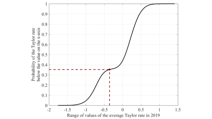
Another way of formulating this monetary policy assessment is to represent the distribution of (average) Taylor rates over a given year. This is shown in Chart 2 for 2019. The black curve represents the probability that the Taylor rate will be lower than the value on the x-axis. For example, in 2019, the probability of a Taylor rate below -1.7% is zero, while the probability of a Taylor rate below 1.5% is 1. The x-axis of the red circle corresponds to the average level of the 3-month Euribor over 2019.

The probability of the Taylor rate being below the average 3-month Euribor is around 35% in 2019. In other words, 35% of Taylor rates are below the average level of the 3-month Euribor in 2019, which suggests that, over the year, monetary conditions were on average very slightly accommodative compared with the distribution of Taylor rates.